Inverting the Steady State of a Markov Chain

Recently while working on a time-series rare-event prediction problem I found myself wanting to generate an infinite stream of training data to test out various prediction approaches. In order to match data from my problem domain, I wanted a model that incorporated a ‘normal’ mode of operation and rare ‘failure’ events, each failure possibly preceded by one or more ‘alarm’ events, and I wanted to be able to create many such models easily. Seemed like a Markov chain would do the trick if I could just figure out a way to go from the desired steady-state distribution to the transition matrix itself. I was actually surprised to find that this is not only possible in many cases, but that the process is relatively simple to understand and to implement with the right tools. More on that later, first let’s review the basics of Markov Chains.

An example of the type of Markov chain I needed to generate.

Markov Chains

Recall that a Markov chain is “a random process that undergoes transitions from one state to another on a state space.” We can represent a Markov chain using a transition matrix, and for our purposes we will use a right-stochastic matrix (meaning that all of its entires are in [0..1] and all of its rows sum to 1.0).

An example transition matrix is given below:

The matrix represents the transition probabilities between the states. If we represent our current state as a vector of probabilities, and represent being in state one by assigning probability 1.0 to the first entry in our state vector, we could compute our next state by multiplying our state vector with the transition matrix (I transposed the vectors here for display purposes only, they are row vectors):

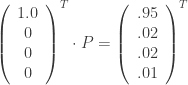
So after one step we have a 95% chance of being in state 1, a 2% chance of being in state 2, a 2% chance of being in state 3, and a 1% chance of being in state 4. To see our chances of being in each state after iterations we can apply the same approach but instead of using , we use . By extension if we take we will get what is called the steady-state vector of the Markov chain. This represents the long-term probabilities of being in a particular state. It is so named because it isn’t changed by the matrix . In other words  is a left-eigenvector of with the eigenvalue of 1.0.

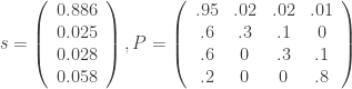
So if we want to represent a rare event preceded by some pre-event states we could model it as a Markov chain using something like the below, where represents the steady state distribution of .

The first row in  represents the ‘normal’ state. It mostly loops back into itself, occasionally transitioning to the other states. The last row is the ‘failure’ state, which mostly loops back to itself, but after a time it will go back to state one. The other two states are a “chain” that links the normal state to the failure state in one or more steps. These chains allow us to gradually move to the  failure mode, which is required to make predicting it possible.

Inverting the Steady State

The main goal here is to create some rare failure event data so we start by choosing  to assign a reasonable amount of probability to state 1 (say 80%) and a very small probability to the failure state (maybe 1e-5). The rest of the probability mass is randomly distributed over the other states. So we have something like this (values rounded for readability):

So the question is, can we build a transition matrix such that is the steady-state vector?

It turns out that this is an under-constrained problem and there may be many solutions, if one exists at all.

Rules of Thumb

1. P must be irreducible – A Markov chain is reducible if a state exists that is inaccessible from some other state .  In other words it has more than one non-communicating equivalence class. A reducible Markov chain will, in general, have multiple steady state distributions. Not good for our purposes.

2. P must be strongly connected – Assuming an irreducible Markov chain, in order for a unique stationary distribution to exist we require that all states be positive recurrent. A state is positive recurrent if the expected value of the recurrence time (the number of transitions until the state is re-entered) is finite. This is equivalent to the requirement that the graph be strongly connected. The graph is strongly connected if every state is reachable from every other state.

3. No zeros in target distribution – Given all of our previous requirements, if a stationary distribution exists for some , then it must be the case that all are strictly positive, so we cannot allow any zeros when setting up our target distribution.

There may be other nuances regarding when this succeeds or fails, but I have found that if I follow these rules this technique works, and works pretty fast, most of the time (once the learning rate is tuned properly).

Cost Function

1. Right Stochastic Constraint – The first thing we need to do is ensure that our matrix  is right-stochastic. That is, its entries are all probabilities and that each row sums to 1.0. Let be a vector of length and let be an matrix.  Then all the rows sum to 1.0 if we can satisfy:

2. All Values Non-Negative – We also need all of our entries to be probabilities. If we assume that the rows sum to one (our previous constraint) then we simply need to ensure that all the entries are non-negative. Let be an indicator function that is equal to 1 if its parameter is negative, and 0 otherwise. Then all our entries are non-negative if we can satisfy:

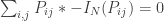
3. Eigenvector – Last, but certainly not least, we want to be an eigenvector of . Rearranging the eigenvector equation we see that this requirement is satisfied by the following:

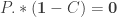
4. Graph Connectivity – The constraints above are good enough to solve the fully connected case, but we will often want to specify a connectivity constraint on our transition matrix. To implement this we use a boolean connectivity matrix which has a 1 for each transition that is legal and a 0 for each transition that is illegal. We invert this matrix and then apply element-wise multiplication, leaving positive penalty values for each illegal transition that has a non-zero probability in .

Now we can define the complete problem as follows:

Since our cost function is differentiable, we can use simple gradient descent to search for a solution (with all the usual caveats). We will use as our parameter and update it using the gradient and a learning rate with the following update rule:

In the next post we will see how to implement a simple solver for this problem in Python and see how to implement graph connectivity constraints as well.